Complex integral contours
Sommerfeld integrals arise in the treatment of the layer system response to the scattered field or to the initial field (in case of dipole excitation). Their numerical evaluation relies on an integral contour that is deflected into the complex plane in order to avoid sharp features stemming from waveguide mode singularities (see the section on Sommerfeld integrals for a short discussion).
Default settings
If you specify no input arguments with regard to the integral contours, default settings are applied. Note, however, that this does not guarantee accurate results in all use cases.
Automatic contour definition
If you want to be on the safe side, use the automatic parameter selection feature to obtain a suitable integral contour, see section on Automatic parameter selection. The drawback is a substantially enhanced runtime, as the simulation is repeated multiple times until the result converges.
Manual contour definition
We recommend to use the neff_imag, neff_max and neff_resolution input parameter of the smuthi.simulation.Simulation constructor.
Smuthi will construct contours based on this input and store them for the duration of the simulation as default contours for multiple scattering and
initial fields in the smuthi.fields module.
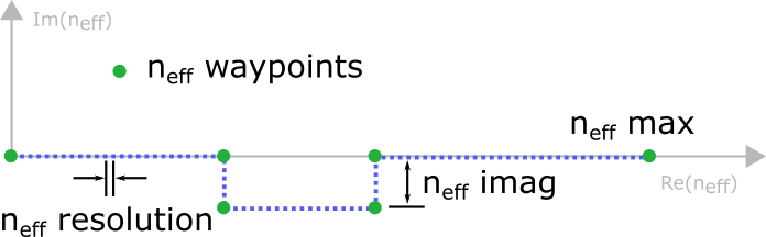
- neff_imag states how far into the negative imaginary the contour will be deflected in terms of the dimensionless effective refractive index, \(n_\mathrm{eff}=\frac{c\kappa}{\omega}\)
- neff_max is the point where the contour ends (on the real axis). Instead of neff_max, you can also provide neff_max_offset which specifies, how far neff_max should be chosen away from the largest relevant layer refractive index.
- neff_resolution denotes the distance \(\Delta n_\mathrm{eff}\) between two adjacent sampling points (again in terms of effective refractive index).
The locations where the waypoints mark a deflection into the imaginary are chosen with consideration of the involved layer system refractive indices (see the section on Sommerfeld integrals for a discussion why that is necessary).
This is how a call to the simulation contructor could look like:
simulation = smuthi.simulation.Simulation( ...
                                          neff_imag=1e-2,
                                          neff_max=2.5,
                                          neff_resolution=5e-3,
                                          ... )
Note
If you need more control over the shape of the contour, read through the API documentation or contact the support mailing list (see Contact).
Multiple scattering and initial field contours
In some use cases it makes sense to specify the contour for multiple scattering with different parameters than the contour for the initial field. For example, when a dipole is very close to an interface, but the particle centers are not.
In that case you can use the function reasonable_Sommerfeld_kpar_contour (see fields)
to construct an array of k_parallel values for each initial field and multiple scattering purposes, like this:
# construct contour arrays
init_kpar = smuthi.fields.reasonable_Sommerfeld_kpar_contour( ... )
scat_kpar = smuthi.fields.reasonable_Sommerfeld_kpar_contour( ... )

# assign them to the respective objects
simulation = smuthi.initial_field.DipoleSource( ...
                                                k_parallel=scat_kpar,
                                                ... )

simulation = smuthi.simulation.Simulation( ...
                                          k_parallel=scat_kpar,
                                          ... )
Guidelines for parameter selection
Contour truncation
The contour truncation scale neff_max is a real number which specifies where the contour ends. It should be larger than the refractive index of the layer in which the particle resides. The offset \(n_\mathrm{eff}-n\) should be chosen with regard to the distance between the particles (and point sources) to the next layer interface. If that distance is large, the truncation scale is uncritical, whereas whereas point sources or particles whose center is very close to a layer interface require a larger offset.
At a \(z\)-distance of \(\Delta z\), evanescent waves with an effective refractive index of \(n_\mathrm{eff}\) are damped by a factor of
where \(\lambda\) is the vacuum wavelength and \(n\) is the refractive index of the medium.
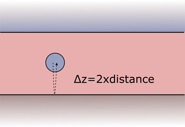
To select a reasonable neff_max, we should consider that the shortest possible interaction path is twice the \(z\)-distance between some particle center (or dipole position) and the next layer interface.
Uncritical example
A layer system consists of a substrate (\(n=1.5\)), covered with a 1000nm thick layer of titania (\(n=2.1\)) under air (\(n=1\)). A silica sphere is immersed in the middle of the titania layer. The system is illuminated with a plane wave at vacuum wavelength of 550nm.
Then, \(\Delta z= 2\times 500\mathrm{nm}\) such that evanescent waves with \(n_\mathrm{eff}=2.3\) are already damped by a factor of \(\exp(-2\pi \frac{1000\mathrm{nm}}{550\mathrm{nm}} \sqrt{(2.3^2-2.1^2)}) \approx 2\times 10^{-5}\) when they propagate to the layer interface and back to the sphere. Waves beyond that effective refractive index thus can be safely neglected in the particle-layer system interaction, such that a truncation parameter of \(n_\mathrm{eff, max}=2.3\) is reasonable.
Critical example
A layer system consists of a substrate (\(n=1.5\)), under air (\(n=1\)). A point dipole source of wavelength 550nm is located 10nm above the substrate/air interface.
Here we need to consider \(\Delta z= 2\times 10\mathrm{nm}\) such that Then, evanescent waves with \(n_\mathrm{eff}=2.3\) are only damped by a factor of \(\exp(-2\pi \frac{20nm}{550nm} \sqrt{(2.3^2-1^2)}) \approx 0.62\) when scattered by the layer interface. Even a truncation of \(n_\mathrm{eff, max}=10\) would only lead to an evanescent damping of \(\exp(-2\pi \frac{20nm}{550nm} \sqrt{(10^2-1^2)}) \approx 0.1\) which might still not be enough.
Resolution
In Smuthi, Sommerfeld integrals are addressed numerical by means of the trapezoidal rule. The discretization of the integrand along the integration contour is determined by the parameter neff_resolution which specifies the distance of one integration node to the next in terms of the effective refractive index. In general, a finer resolution leads to a better accuracy and a longer runtime during preprocessing (i.e., when the particle coupling lookup is computed) as well as during post processing (when the electric field is computed from a plane wave pattern).
The following situations can require a fine sampling of the integrands:
- when a high accuracy is desired
- when waveguide modes and branch point singularities render a numerically challenging integrand of the Sommerfeld integrals (this can be avoided by a deflection into the imaginary, see below)
- when particles with a large distance to each other are part of the simulation geometry
To understand the latter point, consider the Sommerfeld integral as a Hankel transform. Like in a Fourier transform, a large lateral distance requires a fine sampling of the wavenumber to avoid aliasing.
It thus is advised to select neff_resol below \(2 / (k\rho_\mathrm{max})\), where \(k=2\pi/\lambda\) is the vacuum wavenumber and \(\rho_\mathrm{max}\) is the largest lateral distance between two particles.
Deflection into imaginary
Near waveguide mode or branchpoint singularities, the integrand of the Sommerfeld integrals may be a rapidly varying function (in case of lossless media, the waveguide mode singularities are located on the real axis, such that the integrand is even singular). In that case, a deflection of the integral contour into the complex plane can improve the accuracy of the numerical integrals for a given sampling resolution, see also the section on Sommerfeld integrals. The extent of that deflection is set by the neff_imag parameter.
Note
Care has to be taken when selecting the neff_imag parameter, especially in the case of large lateral distances between the particles.
- The larger
neff_imag, the stronger is the smoothing effect on the Sommerfeld integrand - For large lateral distances, a too large
neff_imagcan lead to significant errors! To understand this point, consider the Sommerfeld integral as a Hankel transform, involving expressions of type \(J_\nu(\kappa \rho)\), where \(J_\nu\) is the Bessel function, \(\kappa\) is the in-plane wavenumber (which is proportional to \(n_{\mathrm{eff}}\)) and \(\rho\) is the lateral distance between the particles. Note that the Bessel functions grow rapidly arguments with a large negative imaginary part - which can lead to numerical problems in the integration.
Again, it is thus advised to select neff_imag below \(2 / (k\rho_\mathrm{max})\), where \(k=2\pi/\lambda\) is the vacuum wavenumber and \(\rho_\mathrm{max}\) is the largest lateral distance between two particles.